Amateur Astronomer's Notebook

This article will provide a brief overview of the concept image noise reduction by way of "stacking" images. This article will focus on telescope CCD imaging, however the principles are applicable to many other fields (including Webcam imaging).

Basics

As most amateur CCD imagers know, one of the largest problems with CCD imaging is keeping the background noise in the image to a minimum. All CCD images contain some amount of noise in the image. One method used to reduce noise is to cool the temperature of the CCD chip. This can help greatly in reducing the amount of thermal noise thermal noise that causes CDD images to look less than ideal. However, there are practical limits to the amount of noise reduction that this method can obtain. Another commonly used method to reduce noise is to take multiple images of the same object and then to "stack" the images using the computer. By doing this, the noise in the image will tend to "average out" and the object image will add, resulting in a better signal to noise ratio.

For image stacking to work in an ideal fashion, a few things have to be true:

1. The noise in each image frame must be truly random
2. The "object" being imaged must be the same in each image.

If the above criteria are not met, the amount of image improvement obtained by stacking images will not be ideal.

Some Mathematics…

Consider an image of an astronomical object taken by a CCD camera. This image consists of two portions: signal level due solely to noise and signal level due solely to the object being imaged (a galaxy for example). Ideally we want only the signal that is due to the galaxy. However, it is impossible to determine which part of the total image is due to the galaxy and which part of the total image is due to noise. Fear not, there is some good news. Let's assume we've taken 2 images of the galaxy under the same conditions. In each image, the background noise in the image is random; that is, the noise in image number 1 is different from the noise in image number 2. However, the galaxy in both images is the same. By stacking the two images (which in mathematical terms equates to adding the images) we will see that the galaxy looks better, the noise is reduced (this is noticeable mostly by a decrease in image grain). Why does this work? We shall consider the math below.

Fact Number 1: When random signals are added, the resulting total signal of the sum is the same as the sum of the power of the signals. You may see this referred to in the literature as the incoherent gain of a system

Fact Number 2: When identical signals are added, the signal levels add directly. You may see this referred to in the literature as the coherent gain of a system.

Now, let's take a mathematical look at our images. As noted previously, each image is a combination of signal partly due to noise and partly due to the actual object being imaged (a galaxy in this case). In other words:

Image(total) = image(noise) + image(galaxy).

Now let's add (stack) two images (two different exposures of the same object). The resulting mathematical statement for the new summed image becomes:

Image_new(total) = SQRT(image(noise^2+noise^2)) + 2 x image(galaxy)

This statement may not make much sense just by looking at it. Let's look at some real numbers. For this example, we will keep things simple, we will look at one row of the CCD image. In this case, the CCD chip is 500 pixels by 500 pixels, so we are only going to consider a 1x500 string of data. For simplicity, let's assume that this is an 8 bit CCD camera (output signal range = 0 - 255, where 0 = black and 255 = white). For each of two images, lets say the signal in each pixel (due to the galaxy) is a constant value of 20. Also, let's assume (for each of the two images) that the RMS (root mean squared) value of the noise is also 20. So, for this example, the signal to noise ratio for any one image is 20*log10(signal_value/noise_value) = 20*log10(20/20) = 0. This means that the signal due to the galaxy is the same as that of the noise; in a real world image the galaxy would be on the threshold of visibility in the image. Now let's look at the case of the stacked image. For this case, the summed noise signals produce an RMS level of SQRT(20*20+20*20) = SQRT(800)= 28.28. Notice that the noise signal went up, however it did not double. Now, looking at the summed signal due to the galaxy, we get 2*20 = 40 (notice that in this case the signal does in fact double). So, the signal to noise ratio for this summed image is 20*log10(40/28.28) = 3.01 dB. Thus, by adding the two images, we have increased the signal to noise ratio of the image by 3 dB! We could also say that we have suppressed the noise in the image by 3 dB. Basically, adding images does increase the noise, but the signal increases more, resulting in the better image. In this case the galaxy would stand out a lot better than it would on any one of the individual images, however it would still be a very grainy looking image.

More on Stacking Images

The noise in the image can be further reduced by stacking more images (remember that each image must be a different exposure under the same conditions!). However, due to the way things work in our world, each 3 dB of noise reduction requires that double the number of images be stacked! In other words, stacking two images results in a 3 dB improvement. To get 6 dB requires that 4 images be stacked; to get 9 dB requires that 8 images be stacked! As you can see, this can really add up if you want to get something like a 20 dB improvement!

Visual Examples of Stacking Results

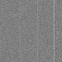
In this section we present images that illustrate the result of stacking various amounts of images. Some things to remember: for stacking to work in an ideal fashion, the noise in each image must be truly random and the signal in each must be identical (otherwise the benefit will be reduced). For this illustration, the "object" being images consists of three lines of various strengths (this was done to keep thing simple). Thirty two individual images were generated (using MATLAB). For each of the 32 images, the background noise is identical in level and random from frame to frame. Also, for each of the 32 images, the signal is identical (the signal levels were set so that at least one of them was pretty well "buried" in noise so that the benefit of stacking can be better shown). To further keep things simple, the final stacked images below are grayscale images (not color). This section shows the results for 6 cases; a single image, and final results for 2, 4, 8, 16 and 32 stacked images. See the table below for more information. Note: the images in the table are .BMP format (JPEG is not suitable for this kind of image).

 

Image	Number of Images Stacked	Signal to Noise Ratio of strongest line (dB)	Notes
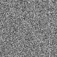	1	0	This image shows a "salt and pepper" characteristic, strongest signal (0db) is barely visible here. The two other signals are at -6 dB and -9 dB, these are totally invisible here. This is a single image, so technically it is not stacked.
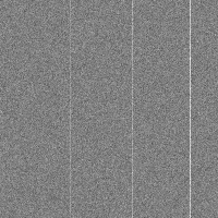
	2	+3	The "salt and pepper" appearance is somewhat muted compared to the previous image. The strongest signal shows better while the two weaker ones (now at - 6dB and 0 dB are showing hints of visibility. In this image the noise has essentially been suppressed by 3 dB as compared to a single frame.
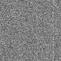
	4	+6	The background noise is beginning to smooth out, some vague traces of the weakest signal (now at 0 dB) are becoming visible. In this image the noise has essentially been suppressed by 6 dB as compared to a single frame.
	8	+9	Background noise is further smoothed, all three signals are now visible (being at +3, +6 and +9dB level now). In this image the noise has essentially been suppressed by 9 dB as compared to a single frame.
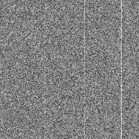
	16	+12	More smoothing of the background, signals are now readily visible. In this image the noise has essentially been suppressed by 12 dB as compared to a single frame.
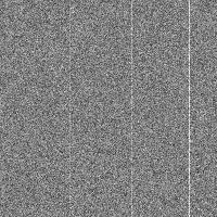
	32	+15	Background noise smoothing out nicely, all signals are easily visible. At this point the signals are not really getting any brighter, they are being "cleaned up" as the noise is suppressed. The weakest signal is now at +6 dB level. In this image the noise has essentially been suppressed by 15 dB as compared to a single frame.

Note that for each successive image the signal to noise ratio gets about 3 dB better. This is because each successive frame above represents a doubling of the number of images stacked.

Some other things to keep in mind (beyond the scope of this article for now): When you stack images, you have to be careful about scaling of the individual images. Scaling refers to the absolute levels of each pixel. As an example of the problem: if your image consists of values greater than 127 (for a 8 bit system), adding two images will cause information to be lost (basically you are clipping the image). The solution is to scale images according to how many you plan to add. Some software programs will do this for you, some will not. In any event, there is more to know about image stacking than is presented here. This article serves primarily to show the principle of how noise reduction works, it does not discuss details of how to actually stack images (another topic for another day...).

%------------------------------ PROGRAM TO SHOW BENEFIT OF IMAGE STACKING --------------------

% March 2001, J. Roberts

% Modified Oct 2003, J. Roberts

% First, generate a 200 x 200 array of random noise.

% Then, add a value of 0.1 to the signal in column 122 (this is our "image" signal)

% Do the same for other columns, make the signal different to show the effect

% Then, make 31 more of these matrixes. The noise in each is different, the signals are

% the same in each...

b=.1; %strength of one line of signal (0.1 =~ -9.1 dB)

a=.145; %.145 =~ -6 dB

c=.29; % .29 =~ 0dB

x1=rand(200,200);

x1(:,122)=x1(:,122)+a;

x1(:,65)=x1(:,65)+b;

x1(:,175)=x1(:,175)+c;

x2=rand(200,200);

x2(:,122)=x2(:,122)+a;

x2(:,65)=x2(:,65)+b;

x2(:,175)=x2(:,175)+c;

x3=rand(200,200);

x3(:,122)=x3(:,122)+a;

x3(:,65)=x3(:,65)+b;

x3(:,175)=x3(:,175)+c;

x4=rand(200,200);

x4(:,122)=x4(:,122)+a;

x4(:,65)=x4(:,65)+b;

x4(:,175)=x1(:,175)+c;

x5=rand(200,200);

x5(:,122)=x5(:,122)+a;

x5(:,65)=x5(:,65)+b;

x5(:,175)=x5(:,175)+c;

x6=rand(200,200);

x6(:,122)=x6(:,122)+a;

x6(:,65)=x6(:,65)+b;

x6(:,175)=x6(:,175)+c;

x7=rand(200,200);

x7(:,122)=x7(:,122)+a;

x7(:,65)=x7(:,65)+b;

x7(:,175)=x7(:,175)+c;

x8=rand(200,200);

x8(:,122)=x8(:,122)+a;

x8(:,65)=x8(:,65)+b;

x8(:,175)=x8(:,175)+c;

x9=rand(200,200);

x9(:,122)=x9(:,122)+a;

x9(:,65)=x9(:,65)+b;

x9(:,175)=x9(:,175)+c;

x10=rand(200,200);

x10(:,122)=x10(:,122)+a;

x10(:,65)=x10(:,65)+b;

x10(:,175)=x10(:,175)+c;

x11=rand(200,200);

x11(:,122)=x11(:,122)+a;

x11(:,65)=x11(:,65)+b;

x11(:,175)=x11(:,175)+c;

x12=rand(200,200);

x12(:,122)=x12(:,122)+a;

x12(:,65)=x12(:,65)+b;

x12(:,175)=x12(:,175)+c;

x13=rand(200,200);

x13(:,122)=x13(:,122)+a;

x13(:,65)=x13(:,65)+b;

x13(:,175)=x13(:,175)+c;

x14=rand(200,200);

x14(:,122)=x14(:,122)+a;

x14(:,65)=x14(:,65)+b;

x14(:,175)=x14(:,175)+c;

x15=rand(200,200);

x15(:,122)=x15(:,122)+a;

x15(:,65)=x15(:,65)+b;

x15(:,175)=x15(:,175)+c;

x16=rand(200,200);

x16(:,122)=x16(:,122)+a;

x16(:,65)=x16(:,65)+b;

x16(:,175)=x16(:,175)+c;

x17=rand(200,200);

x17(:,122)=x17(:,122)+a;

x17(:,65)=x17(:,65)+b;

x17(:,175)=x17(:,175)+c;

x18=rand(200,200);

x18(:,122)=x18(:,122)+a;

x18(:,65)=x18(:,65)+b;

x18(:,175)=x18(:,175)+c;

x19=rand(200,200);

x19(:,122)=x19(:,122)+a;

x19(:,65)=x19(:,65)+b;

x19(:,175)=x19(:,175)+c;

x20=rand(200,200);

x20(:,122)=x20(:,122)+a;

x20(:,65)=x20(:,65)+b;

x20(:,175)=x20(:,175)+c;

x21=rand(200,200);

x21(:,122)=x21(:,122)+a;

x21(:,65)=x21(:,65)+b;

x21(:,175)=x21(:,175)+c;

x22=rand(200,200);

x22(:,122)=x22(:,122)+a;

x22(:,65)=x22(:,65)+b;

x22(:,175)=x22(:,175)+c;

x23=rand(200,200);

x23(:,122)=x23(:,122)+a;

x23(:,65)=x23(:,65)+b;

x23(:,175)=x23(:,175)+c;

x24=rand(200,200);

x24(:,122)=x24(:,122)+a;

x24(:,65)=x24(:,65)+b;

x24(:,175)=x24(:,175)+c;

x25=rand(200,200);

x25(:,122)=x25(:,122)+a;

x25(:,65)=x25(:,65)+b;

x25(:,175)=x25(:,175)+c;

x26=rand(200,200);

x26(:,122)=x26(:,122)+a;

x26(:,65)=x26(:,65)+b;

x26(:,175)=x26(:,175)+c;

x27=rand(200,200);

x27(:,122)=x27(:,122)+a;

x27(:,65)=x27(:,65)+b;

x27(:,175)=x27(:,175)+c;

x28=rand(200,200);

x28(:,122)=x28(:,122)+a;

x28(:,65)=x28(:,65)+b;

x28(:,175)=x28(:,175)+c;

x29=rand(200,200);

x29(:,122)=x29(:,122)+a;

x29(:,65)=x29(:,65)+b;

x29(:,175)=x29(:,175)+c;

x30=rand(200,200);

x30(:,122)=x30(:,122)+a;

x30(:,65)=x30(:,65)+b;

x30(:,175)=x30(:,175)+c;

x31=rand(200,200);

x31(:,122)=x31(:,122)+a;

x31(:,65)=x31(:,65)+b;

x31(:,175)=x31(:,175)+c;

x32=rand(200,200);

x32(:,122)=x32(:,122)+a;

x32(:,65)=x32(:,65)+b;

x32(:,175)=x32(:,175)+c;

% Now, add the images. Make 6 images, one each with 1, 2, 4,8, and 32 images stacked.

% Also, normalize the images (divide each image by the number of images used to generate

% the frame). Also, have MATLAB generate images from the matrices.

noise_sum1=(x1)/1;

imwrite(noise_sum1,'c:\aaa\noise1.bmp','bmp')

noise_sum2=(x1+x2)/2;

imwrite(noise_sum2,'c:\aaa\noise2.bmp','bmp')

noise_sum4=(x1+x2+x3+x4)/4;

imwrite(noise_sum4,'c:\aaa\noise4.bmp','bmp')

noise_sum8=(x1+x2+x3+x4+x5+x6+x7+x8)/8;

imwrite(noise_sum8,'c:\aaa\noise8.bmp','bmp')

noise_sum16=(x1+x2+x3+x4+x5+x6+x7+x8+x9+x10+x11+x12+x13+x14+x15+x16)/16;

imwrite(noise_sum16,'c:\aaa\noise16.bmp','bmp')

noise_sum32=(x1+x2+x3+x4+x5+x6+x7+x8+x9+x10+x11+x12+x13+x14+x15+x16+x17+x18+x19+x20+x21+x22+x23+x24+x25+x26+x27+x28+x29+x30+x31+x32)/32;

imwrite(noise_sum32,'c:\aaa\noise32.bmp','bmp')

%------------------ RMS values -----------

% Find the RMS value of noise in one column of each image

rms(1)=std(noise_sum1(:,1)); % determine the RMS value of the noise in column 1 for the first image

rms(2)=std(noise_sum2(:,1)); % second image

rms(3)=std(noise_sum4(:,1));

rms(4)=std(noise_sum8(:,1));

rms(5)=std(noise_sum16(:,1));

rms(6)=std(noise_sum32(:,1)); % 6th image

rmsa(1)=a/rms(1);

rmsa(2)=a/rms(2);

rmsa(3)=a/rms(3);

rmsa(4)=a/rms(4);

rmsa(5)=a/rms(5);

rmsa(6)=a/rms(6);

rmsb(1)=b/rms(1);

rmsb(2)=b/rms(2);

rmsb(3)=b/rms(3);

rmsb(4)=b/rms(4);

rmsb(5)=b/rms(5);

rmsb(6)=b/rms(6);

rmsc(1)=c/rms(1);

rmsc(2)=c/rms(2);

rmsc(3)=c/rms(3);

rmsc(4)=c/rms(4);

rmsc(5)=c/rms(5);

rmsc(6)=c/rms(6);

rmsa_dB=20*log10(rmsa)

rmsb_dB=20*log10(rmsb)

rmsc_dB=20*log10(rmsc)

rms_dB=20*log10(rms)

"Back" links, e-mail and Copyright

Use your browser's "back" button, or use links below if you arrived here via some other path:

This page is part of the site Amateur Astronomer's Notebook.
E-mail to Joe Roberts
Images and HTML text © Copyright 2001 by Joe Roberts. Please request permission to use photos for purposes other than "personal use".